Note
Click here to download the full example code
How to post-process simulation data
In this example we compute the scattering through an orifice plate in a circular duct with flow. The data is extracted from two Comsol Multiphysics simulations with a similar setup as in this study. The geometry is the same as in this study.
1. Initialization
First, we import the packages needed for this example.
import numpy
import matplotlib.pyplot as plt
import acdecom
The orifice is mounted inside a circular test duct with a radius of 15 mm. The highest frequency of interest is 4000 Hz. The bulk Mach-number is 0.042 and the temperature is 295 Kelvin.
section = "circular"
r = 0.015  # m
f_max = 4000  # Hz
M = 0.042
t = 295  # Kelvin
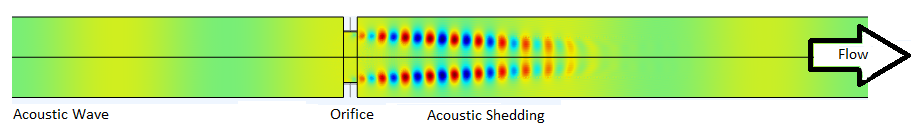
The graphic in the beginning of this examples shows a snapshot of the pressure field from the simulation. The “bubbles” downstream from the orifice plate are the vortex shed by the acoustic field. When we setup the decomposition domain, we want to be outside the shedding region, to avoid detecting artificial modes that do not belong to the acoustic field. Therefore, we will only use pressure values that are at least 10 duct diameters away from the orifice.
distance = 20.*r # m
To analyze the measurement data, we create objects for the US and the DS test ducts.
td_US = acdecom.WaveGuide(dimensions=(r, ), cross_section=section, f_max=f_max, damping="no",
                          M=M, temperature=t, flip_flow=True)
td_DS = acdecom.WaveGuide(dimensions=(r, ), cross_section=section, f_max=f_max, damping="no",
                          M=M, temperature=t)
Note
The standard flow direction is in \(P_+\) direction. On the inlet side, the Mach-number therefore must be either set negative or the argument flipFlow must be set to True.
Note
We use no dissipation model. In the numerical simulation, we have turned off the boundary layer effects and we do not need to take them into account for our post-processing.
2. Data Preparation
We will post-process the direct data output using Comsol Multiphysics. The solution is two-dimensional and axi-symmetric. Using Comsol, we exported the two files comsolOrificeCase1.txt and comsolOrificeCase2.txt. They contain the same geometry. However, the orifice was either excited with an acoustic plane wave from the upstream direction or from the downstream direction. We will post-process both files in order to extract the sound scattering in both directions.
First, we print the header of the files to get a cleaner view of their structure.
with open("data/comsolOrifice1.txt","r") as pressurefile:
    for i in range(11):
        print(pressurefile.readline())
Out:
% Model:              orjfjceWhjstljng2D.mph

% Versjon:            COMSOL 5.5.0.306

% Date:               Jul 23 2020, 09:21

% Djmensjon:          2

% Nodes:              10000

% Expressjons:        71

% Descrjptjon:        Pressure

% Length unjt:        m

% r                       z                        p2 (Pa) @ freq=500                                p2 (Pa) @ freq=550                                p2 (Pa) @ freq=600                                p2 (Pa) @ freq=650                                p2 (Pa) @ freq=700                                p2 (Pa) @ freq=750                                p2 (Pa) @ freq=800                                p2 (Pa) @ freq=850                                p2 (Pa) @ freq=900                                p2 (Pa) @ freq=950                                p2 (Pa) @ freq=1000                               p2 (Pa) @ freq=1050                               p2 (Pa) @ freq=1100                               p2 (Pa) @ freq=1150                               p2 (Pa) @ freq=1200                               p2 (Pa) @ freq=1250                               p2 (Pa) @ freq=1300                               p2 (Pa) @ freq=1350                               p2 (Pa) @ freq=1400                               p2 (Pa) @ freq=1450                               p2 (Pa) @ freq=1500                               p2 (Pa) @ freq=1550                               p2 (Pa) @ freq=1600                               p2 (Pa) @ freq=1650                               p2 (Pa) @ freq=1700                               p2 (Pa) @ freq=1750                               p2 (Pa) @ freq=1800                               p2 (Pa) @ freq=1850                               p2 (Pa) @ freq=1900                               p2 (Pa) @ freq=1950                               p2 (Pa) @ freq=2000                               p2 (Pa) @ freq=2050                               p2 (Pa) @ freq=2100                               p2 (Pa) @ freq=2150                               p2 (Pa) @ freq=2200                               p2 (Pa) @ freq=2250                               p2 (Pa) @ freq=2300                               p2 (Pa) @ freq=2350                               p2 (Pa) @ freq=2400                               p2 (Pa) @ freq=2450                               p2 (Pa) @ freq=2500                               p2 (Pa) @ freq=2550                               p2 (Pa) @ freq=2600                               p2 (Pa) @ freq=2650                               p2 (Pa) @ freq=2700                               p2 (Pa) @ freq=2750                               p2 (Pa) @ freq=2800                               p2 (Pa) @ freq=2850                               p2 (Pa) @ freq=2900                               p2 (Pa) @ freq=2950                               p2 (Pa) @ freq=3000                               p2 (Pa) @ freq=3050                               p2 (Pa) @ freq=3100                               p2 (Pa) @ freq=3150                               p2 (Pa) @ freq=3200                               p2 (Pa) @ freq=3250                               p2 (Pa) @ freq=3300                               p2 (Pa) @ freq=3350                               p2 (Pa) @ freq=3400                               p2 (Pa) @ freq=3450                               p2 (Pa) @ freq=3500                               p2 (Pa) @ freq=3550                               p2 (Pa) @ freq=3600                               p2 (Pa) @ freq=3650                               p2 (Pa) @ freq=3700                               p2 (Pa) @ freq=3750                               p2 (Pa) @ freq=3800                               p2 (Pa) @ freq=3850                               p2 (Pa) @ freq=3900                               p2 (Pa) @ freq=3950                               p2 (Pa) @ freq=4000

7.500000000000002E-4      -0.59895045              -6.594015731195159E-4-9.964393396585407E-4j       -0.0011860537981138028+2.0822981814437445E-4j     -2.812573635939459E-4+0.0011749602856567277j      9.65163291498519E-4+7.295779500173048E-4j         0.0010579064704968448-5.915102194563302E-4j       -1.1299633810741019E-4-0.0012110236740786606j     -0.0011644015797601338-3.8728480818294044E-4j     -8.210587933093777E-4+9.209466744689457E-4j       5.180658103629975E-4+0.0011268455748456206j       0.0012409686455777142-3.272963654214609E-5j       4.740400915810269E-4-0.0011390373155900377j       -8.450716377997362E-4-8.995013121466687E-4j       -0.001169599847273644+4.0110425814857635E-4j      -1.3039831303748967E-4+0.0012465289850809096j     0.0010961551517094925+6.33386654213946E-4j        0.0010449437044638252-7.41766012782377E-4j        -2.3672338342449196E-4-0.0012808716360936038j     -0.0012987480945725624-3.454406262477366E-4j      -9.227312833426118E-4+0.0010964143515957135j      6.862927003256785E-4+0.0013871489725009168j       0.0016607944827237197-1.295756102817592E-4j       4.919128462650932E-4-0.00169648915713534j         -0.0014688616953822992-0.0010823016057667663j     -0.001568971916333237+0.00100217299216616j        3.7564168773138423E-4+0.0018767549272077574j      0.0019516330154208338+3.255542912689751E-4j       9.857703509767491E-4-0.001785248765610653j        -0.001371365248556543-0.0015055457972722754j      -0.0018276254989431557+7.696057665401723E-4j      6.550840143500225E-5+0.0019071981064098945j       0.0017413207893079527+6.364522425065958E-4j       0.0012280725339732749-0.0013566148788370853j      -8.015001573148758E-4-0.0016254122041068062j      -0.0017799442549510831+1.5785775219420768E-4j     -4.8454594201322975E-4+0.0016792859949273694j     0.0013495732542571244+0.001029970253953009j       0.001405996254230656-8.452371419258992E-4j        -2.5203561266966864E-4-0.001567797361693215j      -0.0014983420558976558-3.340089694426043E-4j      -8.257257002655388E-4+0.0012154454801489233j      7.712479784668012E-4+0.00115740452476719j         0.0012876952843918889-2.4592391686245347E-4j      2.742755753953378E-4-0.0012050110194263088j       -9.348915082832261E-4-7.09317490721921E-4j        -9.93247241574712E-4+5.319373712666111E-4j        6.915017202975234E-5+0.0010874313485564335j       9.857681005918568E-4+3.752915489932123E-4j        7.275117798349058E-4-7.167475285822072E-4j        -3.3367704998420904E-4-9.310611528533997E-4j      -9.572825706231807E-4-9.228772847174834E-5j       -4.847697719494012E-4+8.071131767974492E-4j       5.121672883921741E-4+7.76492695449235E-4j         9.179860936588964E-4-1.284257113454432E-4j        2.75136841222777E-4-8.86756471068437E-4j          -6.916919435819609E-4-6.272952084798296E-4j       -8.659481817208404E-4+3.6987286708238824E-4j      -2.042958072472771E-5+9.489871539630312E-4j       8.620807973518022E-4+4.1000280423645236E-4j       7.297379831001061E-4-6.202347678876438E-4j        -2.6537801623804935E-4-9.232939138473764E-4j      -9.554864208060885E-4-1.410769577346627E-4j       -5.294939363672612E-4+8.1919862519288E-4j         5.371274837476116E-4+8.331122667556481E-4j        9.980645644894418E-4-1.5671397363416304E-4j       2.586716091031291E-4-9.948264845250757E-4j        -8.225210499320335E-4-6.390812021337053E-4j       -9.198072939928214E-4+5.099500924965665E-4j       1.0861720927420949E-4+0.001051845546824562j       0.0010120857110790396+3.143191525288762E-4j       6.875837007028902E-4-8.059670838888746E-4j        -4.671443879336398E-4-9.475783524930404E-4j

0.0022500000000000003     -0.59895045              -6.598115227077373E-4-9.966036279599882E-4j       -0.001186282718359856+2.0866397903526702E-4j      -2.8111675933929363E-4+0.0011751987633198313j     9.652398183496232E-4+7.291329745029828E-4j        0.001057923729561758-5.912473327832849E-4j        -1.1326562504414308E-4-0.001211984191634732j      -0.0011653792383793929-3.868434198036737E-4j      -8.238066406174163E-4+9.218457046765307E-4j       5.201400917075564E-4+0.0011263736961986612j       0.0012381928192308606-3.0203811357715177E-5j      4.725440742955169E-4-0.0011381783230260728j       -8.440197961507028E-4-8.98211707781202E-4j        -0.0011704441414358332+3.9915894765788043E-4j     -1.2447948092705977E-4+0.0012431724035378059j     0.0010941192470542518+6.332820372351979E-4j       0.0010450328454385581-7.39583078427309E-4j        -2.3277848835822907E-4-0.0012845399824699616j     -0.0013034745926918823-3.521620533863789E-4j      -9.254949007485222E-4+0.001095703319259605j       6.85619859634462E-4+0.0013902329999068749j        0.001664168514639363-1.2866300962543247E-4j       4.931251526764727E-4-0.0017001298470275474j       -0.0014726758946456658-0.0010838771234689733j     -0.0015710317224750352+0.0010060500868684095j     3.7951733116016467E-4+0.0018793774529327807j      0.0019548210214740064+3.217641649940683E-4j       9.821488423463016E-4-0.0017888990613899882j       -0.0013752913594157722-0.0015023024663686048j     -0.001824993783673856+7.736873527617381E-4j       6.965138246314807E-5+0.001905357699627487j        0.001740344689598924+6.323291627693415E-4j        0.0012240891908249973-0.0013564641818033009j      -8.020846770305993E-4-0.0016217373396053914j      -0.0017767433088535477+1.590587263955981E-4j      -4.828565683612734E-4+0.001676694781004929j       0.001347668543045332+0.0010279374885355666j       0.0014037664128551926-8.440412408293864E-4j       -2.515063082365174E-4-0.0015655089705026788j      -0.001496127636736117-3.3396479775920545E-4j      -8.25225552293132E-4+0.0012134217677317572j       7.694992985756365E-4+0.0011565658802350249j       0.0012866293333335219-2.444889009042483E-4j       2.753948670858984E-4-0.001203815066077736j        -9.336367086660469E-4-7.101497966353269E-4j       -9.93843423941002E-4+5.30671498265087E-4j         6.790079491545605E-5+0.001087846790556794j        9.86045169783435E-4+3.765149082217435E-4j         7.287156555458019E-4-7.169101458836145E-4j        -3.3372744919464884E-4-9.322578087965604E-4j      -9.584832543674161E-4-9.236647436104054E-5j       -4.850057752778102E-4+8.083182216298214E-4j       5.133614902732322E-4+7.769177494798084E-4j        9.186235670945579E-4-1.2957622500132352E-4j       2.7407994082416997E-4-8.876143318356613E-4j       -6.92758352741272E-4-6.263898525091252E-4j        -8.65249732227945E-4+3.711114876052003E-4j        -1.9079356364642515E-5+9.485396673479142E-4j      8.619095645174047E-4+4.086185353649782E-4j        7.284043167159529E-4-6.20339701031345E-4j         -2.6573130198694647E-4-9.220899774393541E-4j      -9.544752497635772E-4-1.4053002986854214E-4j      -5.288276006638048E-4+8.184181638180472E-4j       5.365840898822465E-4+8.324108363466979E-4j        9.974122222583238E-4-1.5638317717412602E-4j       2.5883947790036606E-4-9.94292816627131E-4j        -8.221497702184529E-4-6.391541867643751E-4j       -9.198623231818279E-4+5.097527154440146E-4j       1.0857274989180938E-4+0.0010519562582322634j      0.0010123109841390409+3.142604573046745E-4j       6.874917145292474E-4-8.063419543968825E-4j        -4.67674467303052E-4-9.475314950079873E-4j
There are a few header lines starting with %, followed by the pressure data for different frequencies. The first and second columns are the r and z coordinates of the grid points. The remaining columns hold the pressure at those positions for different frequencies. The frequencies range from 500 Hz to 4000 Hz in steps of 50 Hz. We can create variables that will be useful later in the study.
z_col = 1
r_col = 0
f = numpy.arange(500,4001,50)
header = "%"
Note
There is no column for the circumferential coordinate. The reason is, that we did a two dimensional, axi-symmetric simulation that does not require a circumferential coordinate.
We read both simulation files.
pressure_1 = numpy.loadtxt("data/comsolOrifice1.txt", dtype=complex, comments=header)
pressure_2 = numpy.loadtxt("data/comsolOrifice2.txt", dtype=complex, comments=header)
We delete all positions that are too close to the orifice plate. Furthermore, we split the simulation in upstream (negative z) and downstream (positive z) sides.
pressure_1us = pressure_1[pressure_1[:, z_col] < -distance, :]
pressure_1ds = pressure_1[pressure_1[:, z_col] > distance, :]

pressure_2us = pressure_2[pressure_2[:, z_col] < -distance, :]
pressure_2ds = pressure_2[pressure_2[:, z_col] > distance, :]
We can check how many grid points we have on the upstream and the downstream side.
print("Probes on US side ", pressure_1us.shape[0], ". Probes on DS side: ", pressure_1ds.shape[0])
Out:
Probes on US side 2500 . Probes on DS side: 2500
Generally, we can use all grid points for post processing. However, this is not the best method if we have a large grid with many points. Instead, we will use a random choice of points.
number_of_probes = 100
mics_rows_US = numpy.random.choice(pressure_1us.shape[0], size=number_of_probes, replace=False)
mics_rows_DS = numpy.random.choice(pressure_1ds.shape[0], size=number_of_probes, replace=False)
We extract the coordinates of the random grid points.
z_DS = numpy.abs(pressure_1ds[mics_rows_DS, z_col])  # m
r_DS = numpy.abs(pressure_1ds[mics_rows_DS, r_col])   # m
phi_DS = numpy.zeros((number_of_probes, ))  # deg

z_US = numpy.abs(pressure_1us[mics_rows_US, z_col])  # m
r_US = numpy.abs(pressure_1us[mics_rows_US, r_col])   # m
phi_US = numpy.zeros((number_of_probes, ))  # deg
We assign the random grid points as microphones to the object.
td_US.set_microphone_positions(z_US, r_US, phi_US)
td_DS.set_microphone_positions(z_DS, r_DS, phi_DS)
In order to decompose the simulation data, we must express it in a format that can be processed by
WaveGuide.decompose().
First, we remove all grid points except the random points that we have chosen for the decomposition. Furthermore, we remove the two columns that contain the coordinates of the grid points.
pressure_1us = numpy.delete(pressure_1us[mics_rows_US, :], [z_col,r_col], axis=1)
pressure_1ds = numpy.delete(pressure_1ds[mics_rows_DS, :], [z_col,r_col], axis=1)

pressure_2us = numpy.delete(pressure_2us[mics_rows_US, :], [z_col,r_col], axis=1)
pressure_2ds = numpy.delete(pressure_2ds[mics_rows_DS, :], [z_col,r_col], axis=1)
Next, we add a new row that contains the frequencies (similar to the line in the header of our file), and one
more that contains the test case number. This row is has the value 0 for case 1, and 1 for case 2.
Subsequently, we transpose the array, to have the data format required by WaveGuide.decompose().
pressure_1us = numpy.vstack([pressure_1us, f, numpy.zeros((f.shape[0],))]).T
pressure_2us = numpy.vstack([pressure_2us, f, numpy.ones((f.shape[0],))]).T

pressure_1ds = numpy.vstack([pressure_1ds, f, numpy.zeros((f.shape[0],))]).T
pressure_2ds = numpy.vstack([pressure_2ds, f, numpy.ones((f.shape[0],))]).T
Finally, we combine the two cases at the upstream and the downstream sides to create two large data sets.
pressure_US = numpy.vstack([pressure_1us, pressure_2us])
pressure_DS = numpy.vstack([pressure_1ds, pressure_2ds])
The pressure at the different grid points is stored in the first number_of_probes columns. The frequency is stored in the second last column; and the case number is stored in the last column. We create variables that we will use later in this study.
mic_col = range(0, number_of_probes)
frequ_col = -2
case_col = -1
3. Decomposition
With the pre-processed data, we can run the decomposition.
decomp_us, headers_us = td_US.decompose(pressure_US, frequ_col, mic_col, case_col=case_col)

decomp_DS, headers_DS = td_DS.decompose(pressure_DS, frequ_col, mic_col, case_col=case_col)
4. Further Post-processing
We can print the headersDS to see the names of the columns of the arrays that store the decomposed sound fields.
print(headers_us)
Out:
['(0,0) plus Direction', '(0,0) minus Direction', 'f', 'Mach_number', 'temperature', 'Ps', 'condition number', 'case']
We use that information to extract the modal data.
minusmodes = [1]  # from headers_us
plusmodes = [0]
Furthermore, we acquire the unique decomposed frequency points.
frequs = numpy.abs(numpy.unique(decomp_us[:, headers_us.index("f")]))
nof = frequs.shape[0]
For each of the frequencies we compute the scattering matrix by solving a linear system of equations \(S = p_+ p_-^{-1}\), wherein \(S\) is the scattering matrix and \(p_{\pm}\) are matrices containing the acoustic modes that are placed in rows and the different test cases that are placed in columns.
Note
Details for the computation of the Scattering Matrix and the procedure to measure the different test-cases can be found in this study.
S = numpy.zeros((2,2,nof),dtype = complex)

for fIndx, f in enumerate(frequs):
    frequ_rows = numpy.where(decomp_us[:, headers_us.index("f")] == f)
    ppm_us = decomp_us[frequ_rows]
    ppm_DS = decomp_DS[frequ_rows]
    pp = numpy.concatenate((ppm_us[:,plusmodes].T, ppm_DS[:,plusmodes].T))
    pm = numpy.concatenate((ppm_us[:,minusmodes].T, ppm_DS[:,minusmodes].T))
    S[:,:,fIndx] = numpy.dot(pp, numpy.linalg.pinv(pm))
5. Plot
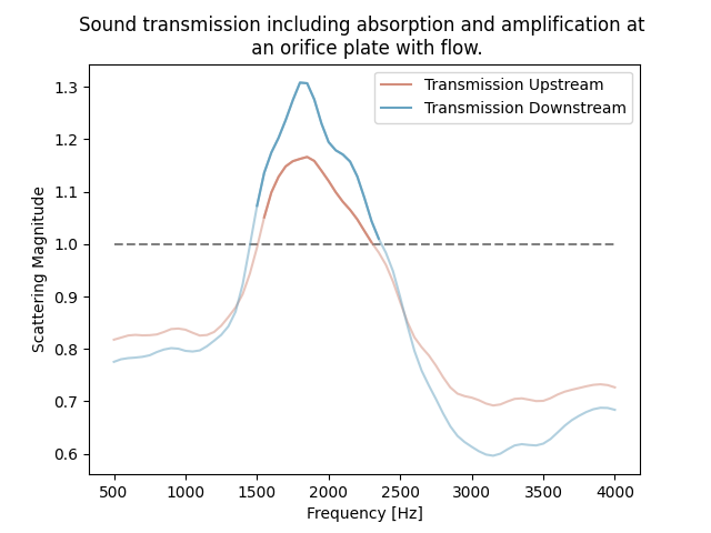
We can plot the transmission coefficients. Transmission coefficients higher than 1 indicate frequencies where amplification can occur.
amplification_us = numpy.abs(S[1, 0, :]) > 1
amplification_ds = numpy.abs(S[0, 1, :]) > 1

plt.hlines(1, frequs[0], frequs[-1], linestyles="dashed", color="grey")

plt.plot(frequs, numpy.abs(S[1, 0, :]),
         ls="-", color="#D38D7B", alpha=0.5)
plt.plot(frequs, numpy.abs(S[0, 1, :]),
         ls="-", color="#67A3C1", alpha=0.5)

plt.plot(frequs[amplification_us], numpy.abs(S[1, 0, amplification_us]),
         ls="-", color="#D38D7B", label="Transmission Upstream")
plt.plot(frequs[amplification_ds], numpy.abs(S[0, 1, amplification_ds]),
         ls="-", color="#67A3C1", label="Transmission Downstream")

plt.xlabel("Frequency [Hz]")
plt.ylabel("Scattering Magnitude")
plt.title("Sound transmission including absorption and amplification at \n an orifice plate with flow.")

plt.legend()
plt.show()
Total running time of the script: ( 0 minutes 3.719 seconds)