How to compute wavenumbers and cut-ons

In this example, the wavenumbers and cut-on modes in a circular waveguide without flow are computed and plotted. The r esults correspondto Rienstra “Fundamentals of Duct Acoustics” (Figures 7 and 8).

1. Initialization

First, we import the packages needed for this example.

import matplotlib.pyplot as plt
import numpy
import acdecom

In this example we compute the wavenumbers for arbitrary mode orders in a circular duct of radius 0.1 m without background flow.

section = "circular"
radius = 1  # [m]
Mach_number = 0

We create an object for our test section. We use the standard conditions for ambient air inside the duct, which are predefined.

td = acdecom.WaveGuide(cross_section = section, dimensions=(radius,), M=Mach_number)

From the td object, we can get the WaveGuide specific properties.

print(td.get_domainvalues())

Out:

{'density': 1.2002432611667804, 'dynamic_viscosity': 1.813e-05, 'specific_heat': 1002.8961443192019, 'heat_capacity': 1.401, 'thermal_conductivity': 0.02587, 'speed_of_sound': 343.35637592387417, 'Mach_number': 0, 'radius': 1, 'bulk-viscosity': 1.0878e-05}

2. Extract the Wavenumbers

We define a non-dimensional frequency from which we compute the maximum frequency for our decomposition.

omega_nondimensional = 20
omega = omega_nondimensional * td.speed_of_sound/radius
f_decomb = omega/(2*numpy.pi)

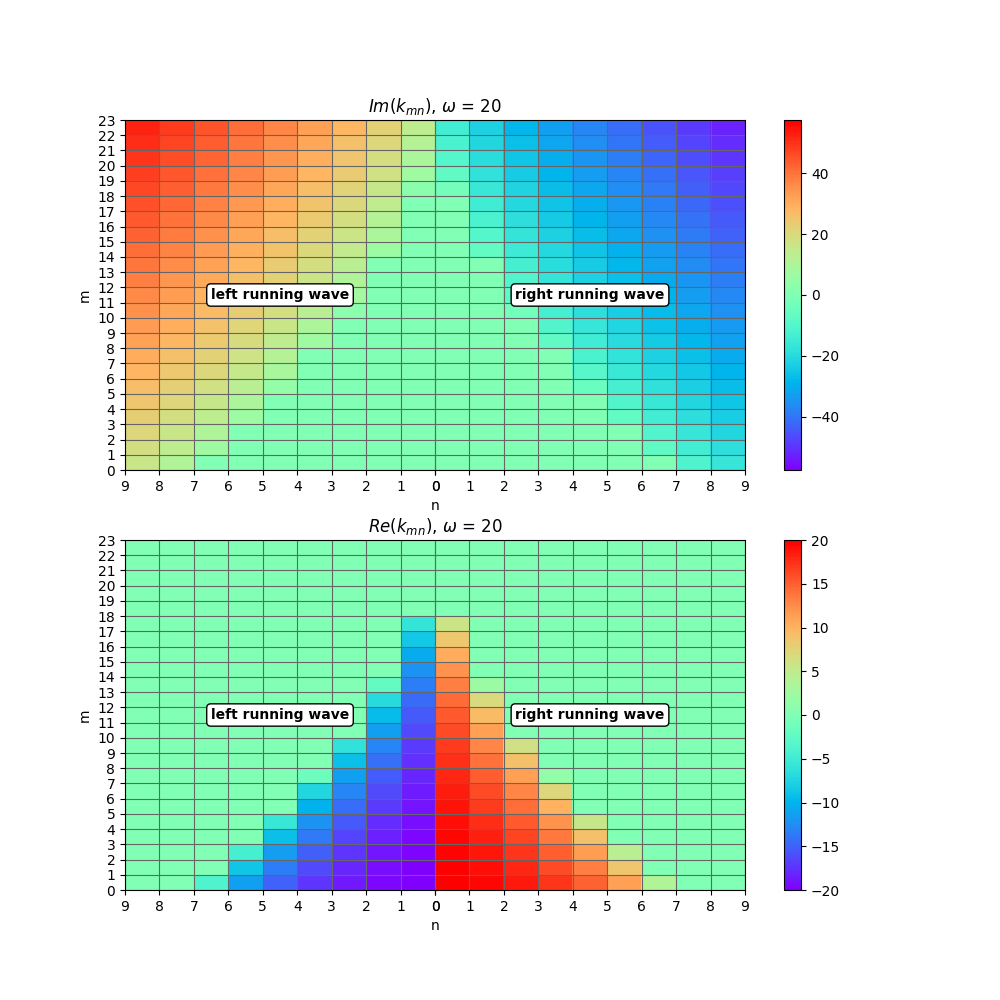
We can conveniently compute the wavenumbers for an arbitrary set of modes by creating two arrays containing all combinations of m and n. In this example we compute the first 24 m modes and the first 10 n modes.

m = numpy.arange(0,24)
n = numpy.arange(0,10)
nn, mm = numpy.meshgrid(n, m)

From the mode arrays we compute the wavenumbers in the left and in the right running direction. We can alter the direction by setting the sign parameter. The \(p_+\) direction has the sign 1 and the \(p_-\) direction has the sign -1.

k_left = td.get_wavenumber(mm, nn, sign = -1, f=f_decomb)
k_right = td.get_wavenumber(mm, nn, sign = 1, f=f_decomb)

3. Plot

Finally, we can plot the real and the imaginary part of the wavenumbers on the m - n grid.

text_params = {'ha': 'center', 'va': 'center', 'family': 'sans-serif',
               'fontweight': 'bold'}
fig, axs = plt.subplots(2,1,figsize = (10,10))
ax=axs[0]
limit = numpy.max(numpy.abs(numpy.imag(k_right)))
kimag_left = ax.pcolor(-n, m, numpy.imag(k_left), cmap="rainbow",vmin=-limit,vmax=limit)
kimag_right = ax.pcolor(n, m, numpy.imag(k_right), cmap="rainbow",vmin=-limit,vmax=limit)
ax.set_xticks(numpy.append(-n,n))
ax.set_yticks(m)
ax.set_xticklabels(numpy.append(n,n))
ax.set_xlabel("n")
ax.set_ylabel("m")
ax.set_title("$Im(k_{mn})$, $\omega$ = "+str(omega_nondimensional))
fig.colorbar(kimag_left, ax=ax)
ax.grid(b=True, which='major', color='#666666', linestyle='-')
ax.text(numpy.max(n)*0.5,numpy.max(m)*0.5,"right running wave",bbox=dict(boxstyle="round",
                   ec="k",fc="w"),**text_params)
ax.text(-numpy.max(n)*0.5,numpy.max(m)*0.5,"left running wave",bbox=dict(boxstyle="round",
                   ec="k",fc="w"),**text_params)
ax=axs[1]
limit = numpy.max(numpy.abs(numpy.real(k_right)))
kimag_left = ax.pcolor(-n, m, numpy.real(k_left), cmap="rainbow",vmin=-limit,vmax=limit)
kimag_right = ax.pcolor(n, m, numpy.real(k_right), cmap="rainbow",vmin=-limit,vmax=limit)
ax.set_xticks(numpy.append(-n,n))
ax.set_xticklabels(numpy.append(n,n))
ax.set_yticks(m)
ax.grid(b=True, which='major', color='#666666', linestyle='-')
ax.text(numpy.max(n)*0.5,numpy.max(m)*0.5,"right running wave",bbox=dict(boxstyle="round",
                   ec="k",fc="w"),**text_params)
ax.text(-numpy.max(n)*0.5,numpy.max(m)*0.5,"left running wave",bbox=dict(boxstyle="round",
                   ec="k",fc="w"),**text_params)
ax.set_xlabel("n")
ax.set_ylabel("m")
ax.set_title("$Re(k_{mn})$, $\omega$ = "+str(omega_nondimensional))
fig.colorbar(kimag_left, ax=ax)
plt.show()

Out:

/home/docs/checkouts/readthedocs.org/user_builds/acdecom/checkouts/latest/examples/plot_RienstraCutOns.py:64: MatplotlibDeprecationWarning: shading='flat' when X and Y have the same dimensions as C is deprecated since 3.3.  Either specify the corners of the quadrilaterals with X and Y, or pass shading='auto', 'nearest' or 'gouraud', or set rcParams['pcolor.shading'].  This will become an error two minor releases later.
  kimag_left = ax.pcolor(-n, m, numpy.imag(k_left), cmap="rainbow",vmin=-limit,vmax=limit)
/home/docs/checkouts/readthedocs.org/user_builds/acdecom/checkouts/latest/examples/plot_RienstraCutOns.py:65: MatplotlibDeprecationWarning: shading='flat' when X and Y have the same dimensions as C is deprecated since 3.3.  Either specify the corners of the quadrilaterals with X and Y, or pass shading='auto', 'nearest' or 'gouraud', or set rcParams['pcolor.shading'].  This will become an error two minor releases later.
  kimag_right = ax.pcolor(n, m, numpy.imag(k_right), cmap="rainbow",vmin=-limit,vmax=limit)
/home/docs/checkouts/readthedocs.org/user_builds/acdecom/checkouts/latest/examples/plot_RienstraCutOns.py:80: MatplotlibDeprecationWarning: shading='flat' when X and Y have the same dimensions as C is deprecated since 3.3.  Either specify the corners of the quadrilaterals with X and Y, or pass shading='auto', 'nearest' or 'gouraud', or set rcParams['pcolor.shading'].  This will become an error two minor releases later.
  kimag_left = ax.pcolor(-n, m, numpy.real(k_left), cmap="rainbow",vmin=-limit,vmax=limit)
/home/docs/checkouts/readthedocs.org/user_builds/acdecom/checkouts/latest/examples/plot_RienstraCutOns.py:81: MatplotlibDeprecationWarning: shading='flat' when X and Y have the same dimensions as C is deprecated since 3.3.  Either specify the corners of the quadrilaterals with X and Y, or pass shading='auto', 'nearest' or 'gouraud', or set rcParams['pcolor.shading'].  This will become an error two minor releases later.
  kimag_right = ax.pcolor(n, m, numpy.real(k_right), cmap="rainbow",vmin=-limit,vmax=limit)

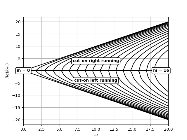
Additionally, we can compute the wavenumbers for a set of modes as a function of the frequency. Again, we create two arrays that contain the combinations of modes. Here, we compute only the m modes and set n to 0.

m = numpy.arange(0, 17)
n = numpy.zeros((m.shape[0],),dtype=int)

We also create an array for the dimensionless frequencies from 0.1 to 20 and allocate arrays for the left and right running wavenumbers.

omegas = numpy.linspace(0.1,20,100)
k_left = numpy.zeros((m.shape[0],omegas.shape[0]))
k_right = numpy.zeros((m.shape[0],omegas.shape[0]))

We iterate through all the dimensionless frequencies and compute the wavenumbers for all modes.

for ii,omega_nondimensional in enumerate(omegas):
    omega = omega_nondimensional * td.speed_of_sound / radius
    f_decomb = omega / (2 * numpy.pi)
    k_left[:,ii] = numpy.real(td.get_wavenumber(m,n,f=f_decomb,sign=-1))
    k_right[:,ii] = numpy.real(td.get_wavenumber(m,n,f=f_decomb,sign=1))

Finally, we plot the results.

plt.figure(2)
for mode in range(k_left.shape[0]):
    plt.plot(omegas,k_right[mode,:],"k")
    plt.plot(omegas, k_left[mode, :], "k")

plt.text(0,0,"m = 0",bbox=dict(boxstyle="round",
                   ec="k",fc="w"),**text_params)
plt.text(numpy.max(omegas)*0.95,0,"m = "+str(numpy.max(m)),
         bbox=dict(boxstyle="round", ec="k",fc="w"),**text_params)
plt.text(numpy.max(omegas)*0.5,numpy.max(k_right)*0.2,"cut-on right running",
         bbox=dict(boxstyle="round", ec="k",fc="w"),**text_params)
plt.text(numpy.max(omegas)*0.5,numpy.min(k_left)*0.2,"cut-on left running",
         bbox=dict(boxstyle="round", ec="k",fc="w"),**text_params)
plt.xlabel("$\omega$")
plt.ylabel("$Re(k_{m0})$")
plt.grid()
plt.xlim(0,numpy.max(omegas))
plt.show()