How to compute wavenumbers in rectangular ducts

In this example we compute the wavenumbers in rectangular ducts without flow. We compare the (mostly-used) Kirchoff dissipation, with the model proposed by Stinson. The Kirchoff model was derived for circular ducts and is adapted to rectangular ducts by computing an equivalent wetted perimeter with the hydraulic radius. The Stinson model is derived for arbitrary cross sections.

1. Initialization

First, we import the packages needed for this example.

import matplotlib.pyplot as plt
import numpy
import acdecom

We create a test duct with a rectangular cross section of the dimensions a = 0.01 m and b = 0.1 m without flow.

section = "rectangular"
a, b = 0.01, 0.1  # [m]
Mach_number = 0

We create two WaveGuides with the predefined dissipation models stinson and kirchoff.

stinson_duct = acdecom.WaveGuide(cross_section=section, dimensions=(a, b), M=Mach_number, damping="stinson")
kirchoff_duct = acdecom.WaveGuide(cross_section=section, dimensions=(a, b), M=Mach_number, damping="kirchoff")

2. Extract the Wavenumbers

We can now loop through the frequencies of interest and compute the wavenumbers for the two WaveGuides.

wavenumber_stinson=[]
wavenumber_kirchoff=[]
frequencies = range(100,2000,50)
m, n = 0, 0
for f in frequencies:
    wavenumber_stinson.append(stinson_duct.get_wavenumber(m, n, f))
    wavenumber_kirchoff.append(kirchoff_duct.get_wavenumber(m, n, f))

3. Plot

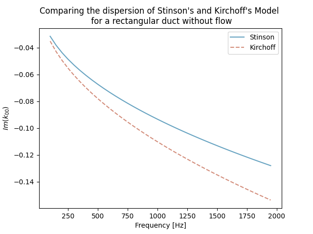
We can plot the imaginary part of the wavenumber, which shows the dissipation of the sound into the surrounding fluid.

plt.plot(frequencies,numpy.imag(wavenumber_stinson), color="#67A3C1", linestyle="-", label="Stinson")
plt.plot(frequencies,numpy.imag(wavenumber_kirchoff), color="#D38D7B", linestyle="--", label="Kirchoff")
plt.legend()
plt.xlabel("Frequency [Hz]")
plt.ylabel("$Im(k_{00})$")
plt.title("Comparing the dispersion of Stinson's and Kirchoff's Model \n for a rectangular duct without flow")
plt.show()

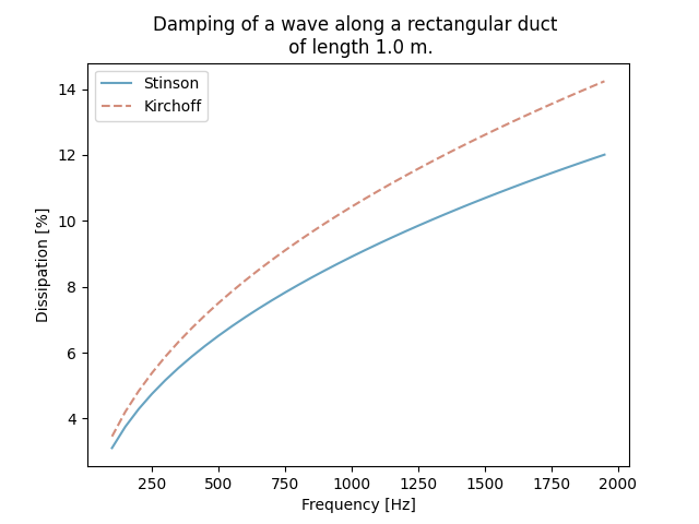
Additionally, we can compute how strongly a wave propagating along a duct of length L is attenuated with the different dissipation models.

L = 10 * b

plt.figure(2)
plt.plot(frequencies,(1-numpy.exp(numpy.imag(wavenumber_stinson)*L))*100, color="#67A3C1", ls="-", label="Stinson")
plt.plot(frequencies,(1-numpy.exp(numpy.imag(wavenumber_kirchoff)*L))*100, color="#D38D7B", ls="--", label="Kirchoff")
plt.xlabel("Frequency [Hz]")
plt.ylabel("Dissipation [%]")
plt.title("Damping of a wave along a rectangular duct \n of length "+str(L)+" m.")
plt.legend()
plt.show()