How to define custom wavenumber functions

In this example we define a custom wavenumber. We inherit from the WaveGuide class and overwrite the internal WaveGuide.get_wavenumber() function. By doing so, we have access to the internal class arguments, such as the domain properties.

1. Inheritance

First, we import the packages needed for the this example.

import matplotlib.pyplot as plt
from matplotlib import cm
import numpy
import acdecom

We create a new class, that we call “slit”. We use the slit class to define a wavenumber for slit-like waveguides within the plane wave range. We implement Stinson’s wavenumber for slits. We inherit from acdecom.testdomain and overwrite two of the methods, namely WaveGuide.get_K0(), which computes the dissipation factor, and WaveGuide.get_eigenvalue(), which computes the Eigenvalue \(\kappa_{m,n}\) that is used to compute the wavenumbers and cut-ons for higher-order modes.

Warning

As the overwritten methods are called by other internal functions, they must have the same positional parameters as their original. Refer to the documentation for more information.

class slit(acdecom.WaveGuide):
    # We inherit all methods and internal variables from *WaveGuide*
    def compute_f(self, x, omega, b):
        return 1 - numpy.tanh(numpy.sqrt(1j * omega * b ** 2 / x)) / numpy.sqrt(1j * omega * b ** 2 / x)
    def get_K0(self,m,n,f,**kwargs):
        # here, we overwrite the function to compute the dissipation factor.
        # We have to use the same  positional parameters as in the original function
        constants = self.get_domainvalues()
        mu = constants["dynamic_viscosity"]
        cp = constants["specific_heat"]
        kth = constants["thermal_conductivity"]
        rho = constants["density"]
        gamma = constants["heat_capacity"]
        b = self.dimensions[0]/2
        omega = 2*numpy.pi*f
        v = mu/rho
        vp = kth/rho/cp
        wavenumber = numpy.sqrt(numpy.array(-(gamma - (gamma - 1) * self.compute_f(vp / gamma, omega, b))
                                            / self.compute_f(v, omega, b), dtype=complex))* -1j

        return wavenumber

    def get_eigenvalue(self, m, n):
        # here we overwrite the function to compute the eigenvalues for the wavenumbers and cut-ons.
        return numpy.pi * (m / self.dimensions[0])

2. Initialization

We create a WaveGuide in slit shape with a dimension of 0.01 m and without flow.

Note

We have to leave the damping argument empty; otherwise our new get_K0 function will be overwritten by a predefined function.

slit_width = 0.01  # m
Mach_number = 0
slit_duct = slit(dimensions=(slit_width,), M=Mach_number)

3. Extract the Wavenumbers

We can now loop through the frequencies of interest and compute the wavenumbers for the slit

wavenumber_slit=[]
frequencies = range(100,2000,50)
m, n = 0, 0

for f in frequencies:
    wavenumber_slit.append(slit_duct.get_wavenumber(m, n, f))

4. Plot

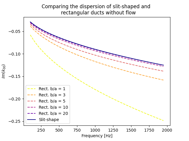
We want to compare the wavenumbers of the slit to the wavenumbers of a rectangular duct with different ratios of slit length and slit width and plot the results

ratio_values = [1, 3, 5, 10, 20]
plt.figure()
colors = cm.plasma_r(numpy.linspace(0,1,len(ratio_values)+1))

for rIndx, ratio in enumerate(ratio_values):
    rect_duct = acdecom.WaveGuide(cross_section="rectangular", dimensions=(slit_width, slit_width*ratio),
                                  damping="stinson")
    wavenumber_rect= []
    for f in frequencies:
        wavenumber_rect.append(rect_duct.get_wavenumber(m, n, f))

    plt.plot(frequencies, numpy.imag(wavenumber_rect), color=colors[rIndx], ls="--", label="Rect. b/a = "+str(ratio))

plt.plot(frequencies, numpy.imag(wavenumber_slit), color=colors[-1], label="Slit-shape")

plt.xlabel("Frequency [Hz]")
plt.ylabel("$Im(k_{00})$")
plt.title("Comparing the dispersion of slit-shaped and \n  rectangular ducts without flow")
plt.legend()
plt.show()