The transmission loss (TL) along a duct liner

In this example we compute the transmission-loss of a duct liner with grazing flow (M=0.25). The data used in this example was part of this study, which is referred to here for further details.

1. Initialization

First, we import the packages needed for this example.

import numpy
import matplotlib.pyplot as plt
import acdecom

The liner is mounted along a duct with a rectangular cross section of the dimensions (0.02 m x 0.11 m). The highest frequency of interest is 1000 Hz. The bulk Mach-number is 0.25 and the temperature is 295 Kelvin.

section = "rectangular"
a = 0.02  # m
b = 0.11  # m
f_max = 1500  # Hz
M = 0.25
t = 295  # Kelvin

Test-ducts were mounted to the downstream and upstream side of the liner. Those ducts were equipped with three microphones, each. The first microphone on each side had a distance of 0.21 m to the liner.

distance_upstream = 0.21  # m
distance_downstream = 0.21  # m

To analyze the measurement data, we create WaveGuide objects for the upstream and the downstream test ducts.

td_upstream = acdecom.WaveGuide(dimensions=(a, b), cross_section=section, f_max=f_max, damping="stinson",
                                distance=distance_upstream, M=M, temperature=t, flip_flow=True)
td_downstream = acdecom.WaveGuide(dimensions=(a, b), cross_section=section, f_max=f_max, damping="stinson",
                                  distance=distance_downstream, M=M, temperature=t)

Note

The standard flow direction is in \(P_+\) direction. Therefore, on the inlet side, the Mach-number must be either set negative or the argument flipFlow must be set to True.

Note

We use Stinson’s model for acoustic dissipation along the pipe. This is more accurate than the model by Kirchoff (which is commonly used). However, it is computationally more expensive.

2. Sensor Positions

We define lists with microphone positions at the upstream and downstream side and assign them to the WaveGuides.

z_downstream = [0, 0.055, 0.248] # m
x_downstream = [a/2, a/2, a/2]  # deg
y_downstream = [0, 0, 0]   # m

z_upstream = [0.249, 0.059, 0]    # m
x_upstream = [a/2, a/2, a/2]  # deg
y_upstream = [0, 0, 0]  # m

td_upstream.set_microphone_positions(z_upstream, x_upstream, y_upstream)
td_downstream.set_microphone_positions(z_downstream, x_downstream, y_downstream)

3. Decomposition

Next, we read the measurement data. The measurement must be pre-processed in a format that is understood by the WaveGuide object. Generally, this is a numpy.ndarray, wherein the columns contain the measurement data, such as the measured frequency and the pressures at the microphone locations. The rows can be different frequencies or different sound excitations (cases). In this example, the measurement was post-processed into the liner.txt file and can be loaded with the numpy.loadtxt function.

Note

The pressure used for the decomposition must be pre-processed, fo example to account for microphone calibration if necessary.

pressure = numpy.loadtxt("data/liner.txt", dtype=complex, delimiter=",", skiprows=1)

We examine the file’s header to understand how the data is stored in our input file.

with open("data/liner.txt") as pressurefile:
    print(pressurefile.readline().split(","))

Out:

['# Mach-Number upstream', 'Mach-Number downstream', 'temperature upstream', 'temperature downstream', 'f', 'Mic1 US', 'Mic2 US', 'Mic3 US', 'Mic1 Liner', 'Mic2 Liner', 'Mic3 Liner', 'Mic4 Liner', 'Mic5 Liner', 'Mic6 Liner', 'Mic7 Liner', 'Mic8 Liner', 'Mic9 Liner', 'Mic10 Liner', 'Mic1 DS', 'Mic2 DS', 'Mic3 DS', 'case\n']

The upstream microphones (1, 2, and 3) are in columns 5, 6, and 7. The Downstream microphones (3, 5, and 6) are in columns 8, 9, and 10. The case number is in the last column. All the other columns contain information that we do not need in this example.

f = 4
mics_ds = [18, 19, 20]
mics_us = [5, 6, 7]
case = -1

Next, we decompose the sound fields into the propagating modes. We decompose the sound fields on the upstream and downstream side of the duct, using the two WaveGuide objects defined earlier.

decomp_us, headers_us = td_upstream.decompose(pressure, f, mics_us, case_col=case)

decomp_ds, headers_ds = td_downstream.decompose(pressure, f, mics_ds, case_col=case)

Note

The decomposition may show warnings for ill-conditioned modal matrices. This typically happens for frequencies close to the cut-on of a mode. However, it can also indicate, that the microphone array is unable to separate the modes. The condition number of the wave decomposition is stored in the data returned by WaveGuide.decompose() and should be checked in case a warning is triggered.

4. Further Post-processing

We can print the headersDS to see the names of the columns of the arrays that store the decomposed sound fields.

print(headers_us)

Out:

['(0,0) plus Direction', '(0,0) minus Direction', 'f', 'Mach_number', 'temperature', 'Ps', 'condition number', 'case']

We use that information to extract the modal data.

minusmodes = [1]  # from headers_us
plusmodes = [0]

Furthermore, we can get the unique decomposed frequency points.

frequs = numpy.abs(numpy.unique(decomp_us[:, headers_us.index("f")]))
nof = frequs.shape[0]

For each of the frequencies, we can compute the scattering matrix by solving a linear system of equations \(S = p_+ p_-^{-1}\), where \(S\) is the scattering matrix and \(p_{\pm}\) are matrices containing the acoustic modes placed in rows and the different test cases placed in columns.

Note

Details for the computation of the Scattering Matrix and the procedure to measure the different test-cases can be found in this study.

S = numpy.zeros((2,2,nof),dtype = complex)

for fIndx, f in enumerate(frequs):
    frequ_rows = numpy.where(decomp_us[:, headers_us.index("f")] == f)
    ppm_us = decomp_us[frequ_rows]
    ppm_ds = decomp_ds[frequ_rows]
    pp = numpy.concatenate((ppm_us[:,plusmodes].T, ppm_ds[:,plusmodes].T))
    pm = numpy.concatenate((ppm_us[:,minusmodes].T, ppm_ds[:,minusmodes].T))
    S[:,:,fIndx] = numpy.dot(pp, numpy.linalg.pinv(pm))

5. Plot

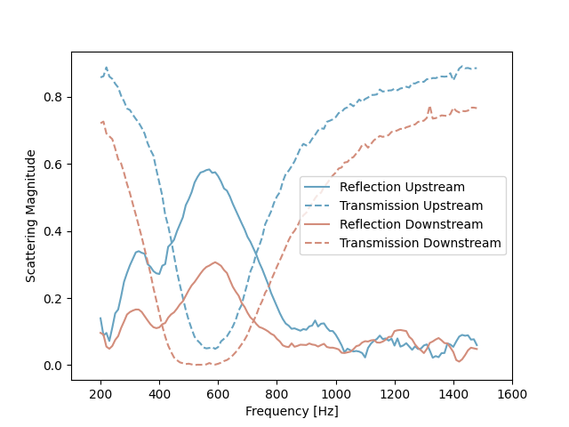
We can plot the transmission and reflection coefficients at the upstream and downstream sides.

plt.plot(frequs, numpy.abs(S[0, 0, :]), ls="-", color="#67A3C1", label="Reflection Upstream")
plt.plot(frequs, numpy.abs(S[1, 0, :]), ls="--", color="#67A3C1", label="Transmission Upstream")
plt.plot(frequs, numpy.abs(S[1, 1, :]), ls="-", color="#D38D7B", label="Reflection Downstream")
plt.plot(frequs, numpy.abs(S[0, 1, :]), ls="--", color="#D38D7B", label="Transmission Downstream")
plt.xlabel("Frequency [Hz]")
plt.ylabel("Scattering Magnitude")
plt.xlim([100,1600])
#plt.ylim([0,1.1])
plt.legend()
plt.show()

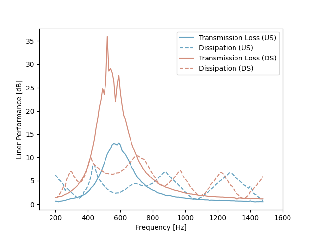
From the scattering matrix, we can compute the transmission loss and the power dissipation of the liner.

TLUpstream = -10* numpy.log10(numpy.abs(S[1, 0, :]))
TLDownstream = -10* numpy.log10(numpy.abs(S[0, 1, :]))

dissipation_us = -10* numpy.log10(numpy.sqrt(numpy.square(S[1, 0, :])+numpy.square(S[0, 0, :])))
dissipation_ds = -10* numpy.log10(numpy.sqrt(numpy.square(S[0, 1, :])+numpy.square(S[1, 1, :])))

plt.plot(frequs, numpy.abs(TLUpstream), ls="-", color="#67A3C1", label="Transmission Loss (US)")
plt.plot(frequs, numpy.abs(dissipation_us), ls="--", color="#67A3C1", label="Dissipation (US)")
plt.plot(frequs, numpy.abs(TLDownstream), ls="-", color="#D38D7B", label="Transmission Loss (DS)")
plt.plot(frequs, numpy.abs(dissipation_ds), ls="--", color="#D38D7B", label="Dissipation (DS)")
plt.xlabel("Frequency [Hz]")
plt.ylabel("Liner Performance [dB]")
plt.xlim([100,1600])
plt.legend()
plt.show()