The empty circular duct with flow and higher-order modes

In this example we extract higher-order modes from measurement data in a circular duct with moderate mean flow. The data is part of this study, which is referred here for further details.

1. Initialization

First, we import the packages needed for this example.

import matplotlib.pyplot as plt
import numpy
import acdecom

The duct has a circular cross section and is filled with air for which we use the standard properties. The duct radius is 0.075 m. The distance from the microphones to the reference cross section is 0.55 m. The highest frequency of interest is 3200 Hz.

section = "circular"
radius = 0.075  # m
distance = 0.55  # [m]
f_max = 3200  # Hz

We create objects for the upstream and the downstream section of the duct.

td_us = acdecom.WaveGuide(dimensions=(radius,), cross_section=section, f_max=f_max, damping="dokumaci",
                          distance=distance, flip_flow=True)
td_ds = acdecom.WaveGuide(dimensions=(radius,), cross_section=section, f_max=f_max, damping="dokumaci",
                          distance=distance)

Note

The standard flow direction is in \(P_+\) direction. On the upstream side, the Mach-number therefore must be either set negative or the argument flip_flow must be set to True.

2. Sensor Positions

The microphone coordinates are saved in the emptyUS.mic and emptyDS.mic file.

td_us.read_microphonefile("data/emptyUS.mic", cylindrical_coordinates=True)
td_ds.read_microphonefile("data/emptyDS.mic", cylindrical_coordinates=True)

Note

In this case, the microphone coordinates are defined in a cylindrical coordinate system with the circumferential position in deg. Therefore, we set the argument cylindrical_coordinates to True. This will transform the circumferential position from deg. to radians.

3. Decomposition

The measurement must be pre-processed in a format that is understood by the WaveGuide object. Generally, this must be a numpy.ndarray, wherein the columns contain the measurement data, such as the measured frequency, the pressure values for that frequency, the bulk Mach-number, and the temperature. The rows can be different frequencies or different sound excitations (cases). In this example, the measurement was post-processed into the higherOrderModes.txt file and can be loaded with the numpy.loadtxt function.

Note

The pressure used for the decomposition must be pre-processed, for example to account for microphone.

pressure = numpy.loadtxt("data/higherOrderModes.txt",dtype=complex, delimiter=",", skiprows=1)

We examine the file header to understand how the data is stored in our input file.

with open("data/higherOrderModes.txt") as pressurefile:
    print(pressurefile.readline().split(","))

Out:

['Mach-Number', 'temperature', 'f', 'Mic1', 'Mic2', 'Mic3', 'Mic4', 'Mic5', 'Mic6', 'Mic7', 'Mic8', 'Mic9', 'Mic10', 'Mic11', 'Mic12', 'Mic13', 'Mic14', 'Mic15', 'Mic16', 'Mic17', 'Mic18', 'Mic19', 'Mic20', 'Mic21', 'Mic22', 'Mic23', 'Mic24', 'case\n']

Mach-number, temperature, and frequency are stored in columns 0, 1, and 2. The upstream microphones 1-12 are in columns 3 - 14, the downstream microphones 13-24 are in columns 15-26, and the case number is in the last column.

Mach_number = 0
temperature = 1
f = 2
mics_us = range(3, 15)
Mics_ds = range(15, 27)
case = -1

Now, we can decompose the sound-fields into the propagating modes. We decompose the sound-fields on the upstream and downstream side of the duct, using the two WaveGuide objects defined earlier.

decomp_us, headers_us = td_us.decompose(pressure, f, mics_us, temperature_col=temperature, case_col=case,
                                        Mach_col=Mach_number)
decomp_ds, headers_ds = td_ds.decompose(pressure, f, Mics_ds, temperature_col=temperature, case_col=case,
                                        Mach_col=Mach_number)

Out:

/home/docs/checkouts/readthedocs.org/user_builds/acdecom/checkouts/latest/src/acdecom.py:1322: UserWarning: The Modal analysis is ill-conditioned for some of the frequencies.
  warnings.warn("The Modal analysis is ill-conditioned for some of the frequencies.")

Note

The decomposition may show warnings for ill-conditioned modal matrices. This typically happens for frequencies close to the cut-on of a mode. However, it can also indicate that the microphone array is insufficient to separate the modes. The condition number of the wave decomposition is stored in the data returned by decompose and should be checked in case a warning is triggered.

4. Further Post-processing

We can print the headers_ds to see the names of the columns of the arrays that store the decomposed sound fields.

print(headers_ds)

Out:

['(0,0) plus Direction', '(-1,0) plus Direction', '(1,0) plus Direction', '(-2,0) plus Direction', '(2,0) plus Direction', '(0,1) plus Direction', '(0,0) minus Direction', '(-1,0) minus Direction', '(1,0) minus Direction', '(-2,0) minus Direction', '(2,0) minus Direction', '(0,1) minus Direction', 'f', 'Mach_number', 'temperature', 'Ps', 'condition number', 'case']

We use that information to extract the modal data for the different frequencies and cases.

plusmodes = [0,1,2,3,4,5]
minusmodes = [6,7,8,9,10,11]

Furthermore, we can get the unique decomposed frequency points.

frequs = numpy.abs(numpy.unique(decomp_us[:,headers_us.index("f")]))
nof = frequs.shape[0]

For each of the frequencies we can compute the scattering matrix by solving a linear system of equations \(S = p_+ p_-^{-1}\), where \(S\) is the scattering matrix and \(p_{\pm}\) are matrices containing the acoustic modes palded in rows and the different test cases placed in columns.

Note

Details for the computation of the Scattering Matrix and the procedure to measure the different test-cases can be found in this study.

S = numpy.zeros((12,12,nof), dtype=complex)
for fIndx, f in enumerate(frequs):
    frequ_rows = numpy.where(decomp_us[:,headers_us.index("f")] == f)
    ppm_us = decomp_us[frequ_rows]
    ppm_ds = decomp_ds[frequ_rows]
    pp = numpy.concatenate((ppm_us[:,plusmodes].T, ppm_ds[:,plusmodes].T))
    pm = numpy.concatenate((ppm_us[:,minusmodes].T, ppm_ds[:,minusmodes].T))
    S[:,:,fIndx] = numpy.dot(pp,numpy.linalg.pinv(pm))

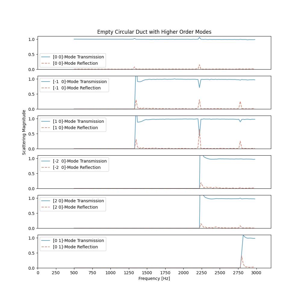
5. Plot

Finally, we can plot the transmission and reflection coefficients of the 6 propagating modes.

mode_names = td_us.mode_vector
fig,axs=plt.subplots(6,1,figsize=(10,10))
axs[0].set_title("Empty Circular Duct with Higher Order Modes")
for mode in range (6):
    axs[mode].plot(frequs, numpy.abs(S[mode,mode+6,:]),
                   color="#67A3C1", label = str(mode_names[mode]) + "-Mode Transmission")
    axs[mode].plot(frequs, numpy.abs(S[mode,mode,:]), ls="--",
                   color="#D38D7B", label = str(mode_names[mode]) + "-Mode Reflection")
    axs[mode].set_xlim([0, 3200])
    axs[mode].set_ylim([0, 1.1])
    axs[mode].set_xticks([])
    axs[mode].legend()

axs[2].set_ylabel("Scattering Magnitude")
axs[5].set_xticks(range(0,3200,250))
plt.xlabel("Frequency [Hz]")
plt.show()