The noise scattering at a compressor inlet and outlet

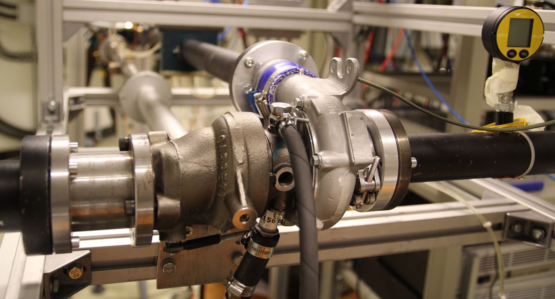
In this example we extract the scattering of noise at a compressor inlet and outlet. In addition to measuring the pressure with flush-mounted microphones, we will use the temperature, and flow velocity that was acquired during the measurement. The data comes from a study performed at the Competence Center of Gas Exchange (CCGEx).

1. Initialization

First, we import the packages needed for this example.

import numpy
import matplotlib.pyplot as plt
import acdecom

The compressor intake and outlet have a circular cross section of the radius 0.026 m and 0.028 m. The highest frequency of interest is 3200 Hz.

section = "circular"
radius_intake = 0.026  # m
radius_outlet = 0.028  # m
f_max = 3200  # Hz

During the test, test ducts were mounted to the intake and outlet. Those ducts were equipped with three microphones each. The first microphone had a distance to the intake of 0.73 m and 1.17 m to the outlet.

distance_intake = 0.073  # m
distance_outlet = 1.17  # m

To analyze the measurement data, we create objects for the intake and the outlet test pipes.

td_intake = acdecom.WaveGuide(dimensions=(radius_intake,), cross_section=section, f_max=f_max, damping="kirchoff",
                              distance=distance_intake, flip_flow=True)
td_outlet = acdecom.WaveGuide(dimensions=(radius_outlet,), cross_section=section, f_max=f_max, damping="kirchoff",
                              distance=distance_outlet)

Note

The standard flow direction is in \(P_+\) direction. Therefore, on the intake side, the Mach-number must be either set negative or the argument flipFlow must be set to True.

2. Sensor Positions

We define lists with microphone positions at the intake and outlet and assign them to the WaveGuides.

z_intake = [0, 0.043, 0.324]  # m
r_intake = [radius_intake, radius_intake, radius_intake]  # m
phi_intake = [0, 180, 0]  # deg

z_outlet = [0, 0.054, 0.284]  # m
r_outlet = [radius_outlet, radius_outlet, radius_outlet]  # m
phi_outlet = [0, 180, 0] #  deg

td_intake.set_microphone_positions(z_intake, r_intake, phi_intake, cylindrical_coordinates=True)
td_outlet.set_microphone_positions(z_outlet, r_outlet, phi_outlet, cylindrical_coordinates=True)

3. Decomposition

Next, we read the measurement data. The measurement must be pre-processed in a format that is understood by the WaveGuide object. This is generally a numpy.ndArray, wherein the columns contain the measurement data, such as the measured frequency, the pressure values for that frequency, the bulk Mach-number, and the temperature. The rows can be different frequencies or different sound excitations (cases). In this example the measurement was post-processed into the turbo.txt file and can be loaded with the numpy.loadtxt function.

Note

The pressure used for the decomposition must be pre-processed, for example to account for microphone calibration.

pressure = numpy.loadtxt("data/turbo.txt",dtype=complex, delimiter=",", skiprows=1)

We review the file’s header to understand how the data is stored in our input file.

with open("data/turbo.txt") as pressure_file:
    print(pressure_file.readline().split(","))

Out:

['# Mach-Number Intake', 'Mach-Number Outlet', 'temperature Intake', 'temperature Outlet', 'f', 'Mic1', 'Mic2', 'Mic3', 'Mic4', 'Mic5', 'Mic6', 'case\n']

The Mach-numbers at the intake and outlet are stored in columns 0 and 1, the temperatures in columns 2 and 3, and the frequency in column 4. The intake microphones (1, 2, and 3) are in columns 5, 6, and 7. The outlet microphones (3, 5, and 6) are in columns 8, 9, and 10. The case number is in the last column.

Machnumber_intake = 0
Machnumber_outlet= 1
temperature_intake = 2
temperature_outlet = 3
f = 4
mics_intake = [5, 6, 7]
mics_outlet = [8, 9, 10]
case = -1

Next, we decompose the sound-fields into the propagating modes. We decompose the sound-fields on the intake and outlet side of the duct, using the two WaveGuide objects defined earlier.

decomp_intake, headers_intake = td_intake.decompose(pressure, f, mics_intake,  temperature_col=temperature_intake,
                                                    case_col=case, Mach_col=Machnumber_intake)

decomp_outlet, headers_outlet = td_outlet.decompose(pressure, f, mics_outlet,  temperature_col=temperature_outlet,
                                                    case_col=case, Mach_col=Machnumber_outlet)

Note

The decomposition may show warnings for ill-conditioned modal matrices. This typically happens for frequencies close to the cut-on of a mode. However, it can also indicate that the microphone array is unable to separate the modes. The condition number of the wave decomposition is stored in the data returned by WaveGuide.decompose() and should be checked in case a warning is triggered.

4. Further Post-processing

We can print the headersDS to see the names of the columns of the arrays that store the decomposed sound fields.

print(headers_intake)

Out:

['(0,0) plus Direction', '(0,0) minus Direction', 'f', 'Mach_number', 'temperature', 'Ps', 'condition number', 'case']

We use that information to extract the modal data.

minusmodes = [1]  # from headers_intake
plusmodes = [0]

Furthermore, we acquire the unique decomposed frequency points.

frequs = numpy.abs(numpy.unique(decomp_intake[:, headers_intake.index("f")]))
nof = frequs.shape[0]

For each of the frequencies, we can compute the scattering matrix by solving a linear system of equations \(S = p_+ p_-^{-1}\), where \(S\) is the scattering matrix and \(p_{\pm}\) are matrices containing the acoustic modes placed in rows and the different test cases placed in columns.

Note

Details for the computation of the Scattering Matrix and the procedure to measure the different test-cases can be found in this study.

S = numpy.zeros((2,2,nof),dtype = complex)

for fIndx, f in enumerate(frequs):
    frequ_rows = numpy.where(decomp_intake[:, headers_intake.index("f")] == f)
    ppm_intake = decomp_intake[frequ_rows]
    ppm_outlet = decomp_outlet[frequ_rows]
    pp = numpy.concatenate((ppm_intake[:,plusmodes].T, ppm_outlet[:,plusmodes].T))
    pm = numpy.concatenate((ppm_intake[:,minusmodes].T, ppm_outlet[:,minusmodes].T))
    S[:,:,fIndx] = numpy.dot(pp,numpy.linalg.pinv(pm))

5. Plot

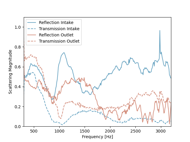
Finally, we can plot the transmission and reflection coefficients at the intake and outlet.

plt.plot(frequs, numpy.abs(S[0, 0, :]), ls="-", color="#67A3C1", label="Reflection Intake")
plt.plot(frequs, numpy.abs(S[0, 1, :]), ls="--", color="#67A3C1", label="Transmission Intake")
plt.plot(frequs, numpy.abs(S[1, 1, :]), ls="-", color="#D38D7B", label="Reflection Outlet")
plt.plot(frequs, numpy.abs(S[1 ,0, :]), ls="--", color="#D38D7B", label="Transmission Outlet")
plt.xlabel("Frequency [Hz]")
plt.ylabel("Scattering Magnitude")
plt.xlim([300,3200])
plt.ylim([0,1.1])
plt.legend()
plt.show()